
PyNGL > tutorial examples > 1 | 2 | 3 | 4 | 5 | 6 | 7 | 8 | 9 | 10 | 11
Example 2 - Contour plots
This example reads a netCDF file and creates five contour plots using three different datasets, and it sets resources to get different types of contour plots. This example also writes some of the netCDF data to an ASCII file.To find out more about netCDF, see http://my.unidata.ucar.edu/content/software/netcdf/
To run this example, you must have Numerical Python installed in your Python implementation. Numerical Python (also known as "NumPy") is a Python module allowing for efficient array processing.
This example reads in a netCDF file, so you will need to have the Nio module (this module comes with PyNGL). netCDF is a self-documenting and network-transparent data format - see the netCDF User Guide for details.
There are two ways to run this example:
execute
pynglex ngl02p
or
download
ngl02p.pyand type:
python ngl02p.py
Output from example 2
| Frame 1 | Frame 2 | Frame 3 | Frame 4 | Frame 5 |
|---|---|---|---|---|
| 
| 
| 
| 
|
(Click on any frame to see it enlarged.)
  0. #
  1. #  Import Python modules to be used.
  2. #
  3. import numpy,sys,os
  4.
  5. #
  6. #  Import Nio (for reading netCDF files).
  7. #
  8. import Nio
  9.
 10. #
 11. #  Import Ngl support functions.
 12. #
 13. import Ngl
 14.
 15. #
 16. #  Open the netCDF file.
 17. #
 18. cdf_file = Nio.open_file(Ngl.pynglpath("data") + "/cdf/contour.cdf","r")
 19.
 20. #
 21. #  Associate Python variables with NetCDF variables.
 22. #  These variables have associated attributes.
 23. #
 24. temp = cdf_file.variables["T"]    # temperature
 25. Z    = cdf_file.variables["Z"]    # geopotential height
 26. pres = cdf_file.variables["Psl"]  # pressure at mean sea level
 27. lat  = cdf_file.variables["lat"]  # latitude
 28. lon  = cdf_file.variables["lon"]  # longitude
 29.
 30. #
 31. #  Open a workstation and specify a different color map.
 32. #
 33. wkres = Ngl.Resources()
 34. wkres.wkColorMap = "default"
 35. wks_type = "ps"
 36. wks = Ngl.open_wks(wks_type,"ngl02p",wkres)
 37.
 38. resources = Ngl.Resources()
 39. #
 40. #  Define a NumPy data array containing the temperature for the
 41. #  first time step and first level. This array does not have the
 42. #  attributes that are associated with the variable temp.
 43. #
 44. tempa = temp[0,0,:,:]
 45.
 46. #
 47. #  Convert tempa from Kelvin to Celcius while retaining the missing values.
 48. #  If you were to write the new temp data to a netCDF file, then you
 49. #  would want to change the temp units to "(C)".
 50. #
 51. if hasattr(temp,"_FillValue"):
 52.   tempa = ((tempa-273.15)*numpy.not_equal(tempa,temp._FillValue)) +   \
 53.         temp._FillValue*numpy.equal(tempa,temp._FillValue)
 54. else:
 55.   tempa = tempa - 273.15
 56.
 57. #
 58. #  Set the scalarfield missing value if temp has one specified.
 59. #
 60. if hasattr(temp,"_FillValue"):
 61.   resources.sfMissingValueV = temp._FillValue[0]
 62.
 63. #
 64. #  Specify the main title base on the long_name attribute of temp.
 65. #
 66. if hasattr(temp,"long_name"):
 67.   resources.tiMainString = temp.long_name
 68.
 69. plot = Ngl.contour(wks,tempa,resources)
 70.
 71. #----------- Begin second plot -----------------------------------------
 72.
 73. resources.cnMonoLineColor = False  # Allow multiple colors for contour lines.
 74. resources.tiMainString    = "Temperature (C)"
 75.
 76. plot = Ngl.contour(wks,tempa,resources)  # Draw a contour plot.
 77.
 78. #----------- Begin third plot -----------------------------------------
 79.
 80. resources.cnFillOn          = True    # Turn on contour line fill.
 81. resources.cnMonoFillPattern = False   # Turn off using a single fill pattern.
 82. resources.cnMonoFillColor   = True
 83. resources.cnMonoLineColor   = True
 84.
 85. if hasattr(lon,"long_name"):
 86.   resources.tiXAxisString = lon.long_name
 87. if hasattr(lat,"long_name"):
 88.   resources.tiYAxisString = lat.long_name
 89. resources.sfXArray        = lon[:]
 90. resources.sfYArray        = lat[:]
 91. resources.pmLabelBarDisplayMode = "Never" # Turn off label bar.
 92.
 93. plot = Ngl.contour(wks,tempa,resources)   # Draw a contour plot.
 94.
 95. #---------- Begin fourth plot ------------------------------------------
 96.
 97. #
 98. #  Specify a new color map.
 99. #
100. rlist = Ngl.Resources()
101. wkres.wkColorMap = "BlGrYeOrReVi200"
102. Ngl.set_values(wks,rlist)
103.
104. resources.cnMonoFillPattern     = True     # Turn solid fill back on.
105. resources.cnMonoFillColor       = False    # Use multiple colors.
106. resources.cnLineLabelsOn        = False    # Turn off line labels.
107. resources.cnInfoLabelOn         = False    # Turn off informational
108.                                              # label.
109. resources.pmLabelBarDisplayMode = "Always" # Turn on label bar.
110. resources.cnLinesOn             = False    # Turn off contour lines.
111.
112. resources.tiMainFont      = 26
113. resources.tiXAxisFont     = 26
114. resources.tiYAxisFont     = 26
115.
116. if hasattr(Z,"_FillValue"):
117.   resources.sfMissingValueV = Z._FillValue
118. if hasattr(Z,"long_name"):
119.   resources.tiMainString = Z.long_name
120. plot = Ngl.contour(wks,Z[0,0,:,:],resources)    # Draw a contour plot.
121.
122. #---------- Begin fifth plot ------------------------------------------
123.
124. cmap = numpy.array([[0.00, 0.00, 0.00], [1.00, 1.00, 1.00], \
125.                     [0.10, 0.10, 0.10], [0.15, 0.15, 0.15], \
126.                     [0.20, 0.20, 0.20], [0.25, 0.25, 0.25], \
127.                     [0.30, 0.30, 0.30], [0.35, 0.35, 0.35], \
128.                     [0.40, 0.40, 0.40], [0.45, 0.45, 0.45], \
129.                     [0.50, 0.50, 0.50], [0.55, 0.55, 0.55], \
130.                     [0.60, 0.60, 0.60], [0.65, 0.65, 0.65], \
131.                     [0.70, 0.70, 0.70], [0.75, 0.75, 0.75], \
132.                     [0.80, 0.80, 0.80], [0.85, 0.85, 0.85]],'f')
133.
134. rlist.wkColorMap = cmap
135. Ngl.set_values(wks,rlist)
136.
137. #
138. #  If the pressure field has a long_name attribute, use it for a title.
139. #
140. if hasattr(pres,"long_name"):
141.   resources.tiMainString = pres.long_name
142.
143. #
144. #  Convert the pressure to millibars while retaining the missing values.
145. #
146. presa = pres[0,:,:]
147. if hasattr(pres,"_FillValue"):
148.   presa = (0.01*presa*numpy.not_equal(presa,pres._FillValue)) +   \
149.         pres._FillValue*numpy.equal(presa,pres._FillValue)
150. else:
151.   presa = 0.01*presa
152.
153. plot = Ngl.contour(wks,presa,resources)  # Draw a contour plot.
154.
155. print "\nSubset [2:6,7:10] of temp array:" # Print subset of "temp" variable.
156. print tempa[2:6,7:10]
157. print "\nDimensions of temp array:"        # Print dimension names of T.
158. print temp.dimensions
159. print "\nThe long_name attribute of T:"    # Print the long_name attribute of T.
160. print temp.long_name
161. print "\nThe nlat data:"                   # Print the lat data.
162. print lat[:]
163. print "\nThe nlon data:"                   # Print the lon data.
164. print lon[:]
165.
166. #
167. #  Write a subsection of tempa to an ASCII file.
168. #
169. os.system("/bin/rm -f data.asc")
170. sys.stdout = open("data.asc","w")
171. for i in range(7,2,-2):
172.   for j in range(0,5):
173.     print "%9.5f" % (tempa[i,j])
174.
175. # Clean up (not really necessary, but a good practice).
176.
177. del plot
178. del resources
179. del temp
180.
181. Ngl.end()
Explanation of example 2
Line 3:
import numpy,sys,os
Import the Numerical Python module. You must have this module installed in your Python implementation. This module is used for efficient array processing. The names of the functions in the Numerical Python package are not exposed by this import, meaning that all functions and attributes in that package will have to be qualified with "numpy".
The Numerical Python package is also known as "NumPy". The Python modules os and sys will also be used in this example.
import Nio
Import the Nio module for a netCDF reader. This module comes with the PyNGL package. netCDF is a self-documenting and network-transparent data format - see the netCDF User Guide for details.
Note: you can also use the netCDF module from the ScientificPython package to read netCDF files. To do this, you need to install ScientificPython, and then import the module:
from Scientific.IO.NetCDF import NetCDFFile
import Ngl
Import all of the Ngl functions. The Ngl module must be on your Python search path.
cdf_file = Nio.open_file(Ngl.ncargpath("data") + "/cdf/contour.cdf","r")
The built-in function Ngl.pynglpath returns the full pathname for a given PyNGL system directory, or the default value for a particular internal parameter.
To use the netCDF module from the ScientificPython package to read the netcdf file, change "Nio.open_file" to "NetCDFFile".
  temp = cdf_file.variables["T"]    # temperature
  Z    = cdf_file.variables["Z"]    # geopotential height
  pres = cdf_file.variables["Psl"]  # pressure at mean sea level
  lat  = cdf_file.variables["lat"]  # latitude
  lon  = cdf_file.variables["lon"]  # longitude
These assignments associate Python NumPy objects with netCDF variables. No data is actually read in making these assignments.
  wkres = Ngl.Resources()
  wkres.wkColorMap = "default"
  wks_type = "ps"
  wks = Ngl.open_wks(wks_type,"ngl02p",wkres)
Open a workstation for drawing the contour plots, and use a resource list to change the colormap to one called "default". The creation of a resource list will be described in the next section.
resources = Ngl.Resources()
A resource list will be used to change the look of the plot (see example 1 for an explanation on how resources are set). Contour plot resources are part of the "ContourPlot" group and all start with the letters "cn". They are documented in the ContourPlot resource descriptions section.
Data associated with a contour plot is called a "ScalarField." ScalarField resources start with "sf" and are documented in the ScalarField resource descriptions section.
tempa = temp[0,0,:,:]
Define a NumPy data array containing the temperature for the first time step and first level. This assignment reads the specified data into the NumPy array tempa. This array does not have the attributes that are associated with the variable temp.
  if hasattr(temp,"_FillValue"):
    tempa = ((tempa-273.15)*numpy.not_equal(tempa,temp._FillValue)) +   \
          temp._FillValue*numpy.equal(tempa,temp._FillValue)
  else:
    tempa = tempa - 273.15
These calculations convert the tempa array from Kelvin to Celcius. If temp has a _FillValue set, then we have to make sure that those values are not converted; if temp does not have a _FillValue set, then the conversion can be done without care for missing values.
  if hasattr(temp,"_FillValue"):
    resources.sfMissingValueV = temp._FillValue[0]
Specify the missing value for the scalar filed data if there is one. The Ngl.contour function will ignore missing value data.
  if hasattr(temp,"long_name"):
    resources.tiMainString = temp.long_name
If the temperature variable in the netCDF file has a long_name attribute, then use that for the main plot title.
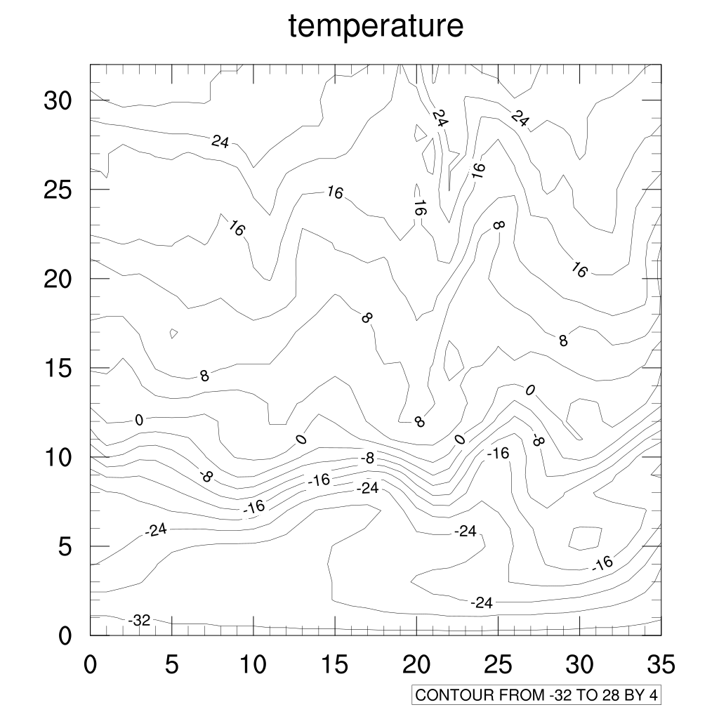
plot = Ngl.contour(wks,tempa,resources)
Create and draw a contour plot of the 2-dimensional array tempa. The first argument of the Ngl.contour function is the workstation object returned from the previous call to Ngl.open_wks. The next argument is the 2-dimensional NumPy scalar field to be contoured, which can be of the NumPy float, double, or integer types. The first dimension must be the Y dimension, and the second the X. The last argument is a resource list.
The default contour plot drawn contains labeled tick marks and an "informational" label at the bottom right of the plot, indicating the range and spacing of the contour levels. Later examples show how to turn this informational label off, and how to customize the tick marks. Also, since no ranges have been defined for the X and Y axes in this plot, the range values default to 0 to n-1, where n is the number of points in that dimension.
resources.cnMonoLineColor = False # Allow multiple colors for contour lines.
Occasionally you will see resource names with the word "Mono" in them. In this case, by setting cnMonoLineColor to False, you are telling PyNgl that you don't want to use a single color for all the contour lines, so it uses the "plural" resource cnLineColors to determine the line color for each line. If cnMonoLineColor had been set to True, then all contour lines would have been drawn in the same color determined by the "singular" resource cnLineColor.
The cnLineColors resource is an example of a resource that is set dynamically when you run the PyNGL script. PyNGL determines how many contour levels you have, then sets cnLineColors with enough color indices to color each line.
resources.tiMainString = "Temperature (C)"
Create a title for the second plot (thus overriding the default title provided by the "long_name" attribute).
plot = Ngl.contour(wks,tempa,resources) # Draw a contour plot.
Draw a new contour plot using the resources you just set.
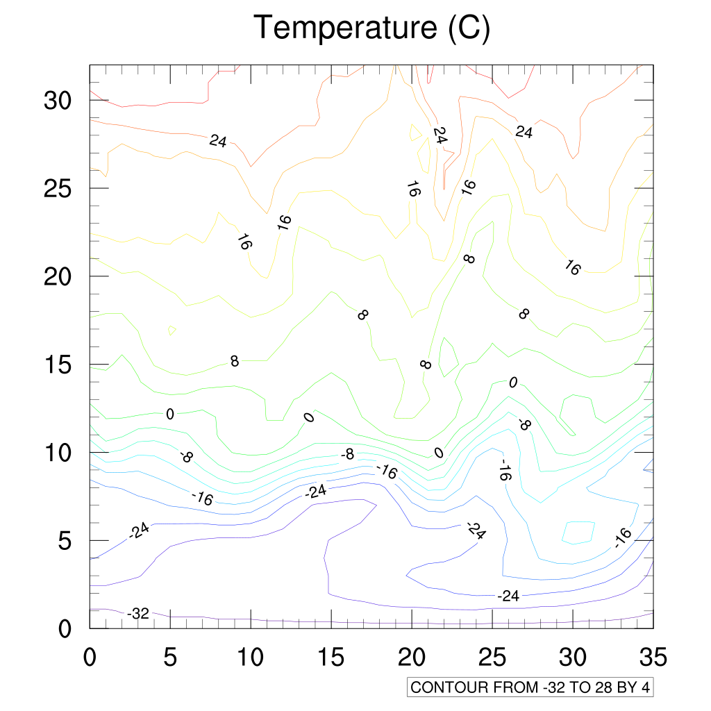
#----------- Begin third plot -----------------------------------------
Draw the same contour plot, only this time fill the contours with the default hatching patterns. Also, explicitly define the ranges for the X and Y axes.
  resources.cnFillOn          = True    # Turn on contour line fill.
  resources.cnMonoFillPattern = False   # Turn off using a single fill pattern.
  resources.cnMonoFillColor   = True
  resources.cnMonoLineColor   = True
By default, contour levels are not filled, so to get filled contours you need to set the resource cnFillOn to True. Also by default, when you fill contour levels, they are all filled in a solid color, so you need to set cnMonoFillPattern to False, telling PyNGL to use different fill patterns for each contour level.
A default set of fill patterns is provided dynamically through the cnFillPatterns resource. There are 17 different fill patterns available, each one represented by an integer from 1 to 17 (0 represents solid fill). So, to change the fill patterns, set the cnFillPatterns resource to an integer array with the same number of elements as you have contour levels.
You can see all the available fill patterns in the "Fill patterns" section.
By setting cnMonoFillColor and cnMonoLineColor both to True, you are telling PyNGL to use the same color for all the fills and lines (the default is the foreground color).
  if hasattr(lon,"long_name"):
    resources.tiXAxisString = lon.long_name
  if hasattr(lat,"long_name"):
    resources.tiYAxisString = lat.long_name
Create labels for the X and Y axes in the contour plot, using the attribute long_name defined for both lat and lon.
  resources.sfXArray        = lon[:]
  resources.sfYArray        = lat[:]
By setting the ScalarField resources sfXArray and sfYArray to the 1-dimensional arrays lon and lat, you can explicitly define the range for the X and Y axes.
resources.pmLabelBarDisplayMode = "Never" # Turn off label bar.
Do not display a label bar.
plot = Ngl.contour(wks,tempa,resources) # Draw a contour plot.
Draw the contour plot. Note the new ranges for the X and Y axes, and the new title and X/Y axis labels.
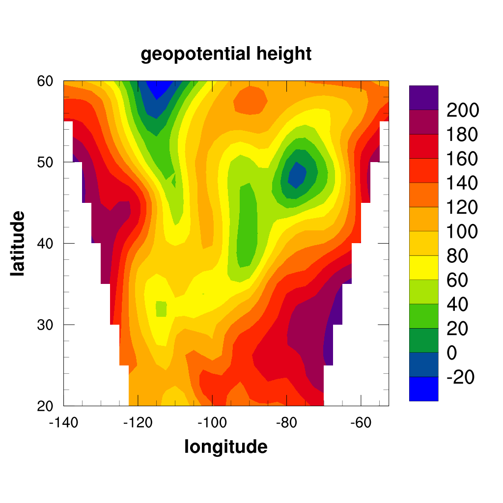
#---------- Begin fourth plot ------------------------------------------
Draw a contour plot of the Z variable, fill the contour lines in solid colors and add a label bar on the side.
  rlist = Ngl.Resources()
  wkres.wkColorMap = "BlGrYeOrReVi200"
  Ngl.set_values(wks,rlist)
The PyNGL function Ngl.set_values allows you to set values of resources associated with an object after it has been created. In the case here we are assigning a new color map called "BlGrYeOrReVi200" to the workstation where the plots are being drawn.
  resources.cnMonoFillPattern     = True     # Turn solid fill back on.
  resources.cnMonoFillColor       = False    # Use multiple colors.
  resources.cnLineLabelsOn        = False    # Turn off line labels.
  resources.cnInfoLabelOn         = False    # Turn off informational
                                               # label.
To fill the contours with solid fill in different colors, you need to set cnMonoFillPattern back to True, telling Ngl.contour to use solid fills for all contour levels, and cnMonoFillColor to False to get multiple fill colors. The other resources turn off the labeling of contour lines, and the "informational" label you saw at the lower right corner in the previous contour plots.
  resources.pmLabelBarDisplayMode = "Always" # Turn on label bar.
  resources.cnLinesOn             = False    # Turn off contour lines.
There are times when you want to add other graphical objects to a plot, like a label bar, a legend, tick marks, or a title. In PyNGL, there's something called a PlotManager that lets you do this. It's called this because it "manages" the look of these additional objects and tries to make intelligent guesses about where the additional objects should be drawn with respect to the original plot. Also, if you resize the original plot, then these extra objects get resized as well. Some of these objects are always drawn by default, like tick marks and a title (if you specify one). A label bar is not drawn by default, so you need to tell the PlotManager to draw it by setting the PlotManager resource pmLabelBarDisplayMode to the predefined string "Always" (the default is "Never"). PlotManager resources start with "pm", and label bar resources start with "lb". These resources are documented in the Labelbar resource descriptions and "PlotManager" resource descriptions sections.
As noted in example 1, predefined strings are case-insensitive, so the pmLabelBarDisplayMode resource could have also been set using "always" or "ALWAYS" or any another combination of uppercase and lower case characters.
The resource cnLinesOn controls whether contour lines are drawn.
  resources.tiMainFont      = "Helvetica-bold"
  resources.tiXAxisFont     = "Helvetica-bold"
  resources.tiYAxisFont     = "Helvetica-bold"
Change the fonts of the title and the X and Y axis labels. A table of all the available fonts with their index values appears in the "Font table" section. In this case, you are changing the font to "Helvetica-bold."
  if hasattr(Z,"_FillValue"):
    resources.sfMissingValueV = Z._FillValue
Specify the missing value for the scalar field data.
  if hasattr(Z,"long_name"):
    resources.tiMainString = Z.long_name
Set the main title using the long_name attribute of Z.
plot = Ngl.contour(wks,Z[0,0,:,:],resources) # Draw a contour plot.
Draw the fourth contour plot with a new dataset. Note that there are some areas in the contour plot that aren't being drawn. This is due to the presence of missing values in the data. By default, if the data being passed to any of the Ngl.* plotting routines contains the attribute "_FillValue," then the user must inform the appropriate object of this value as we have done here with sfMissingValueV.
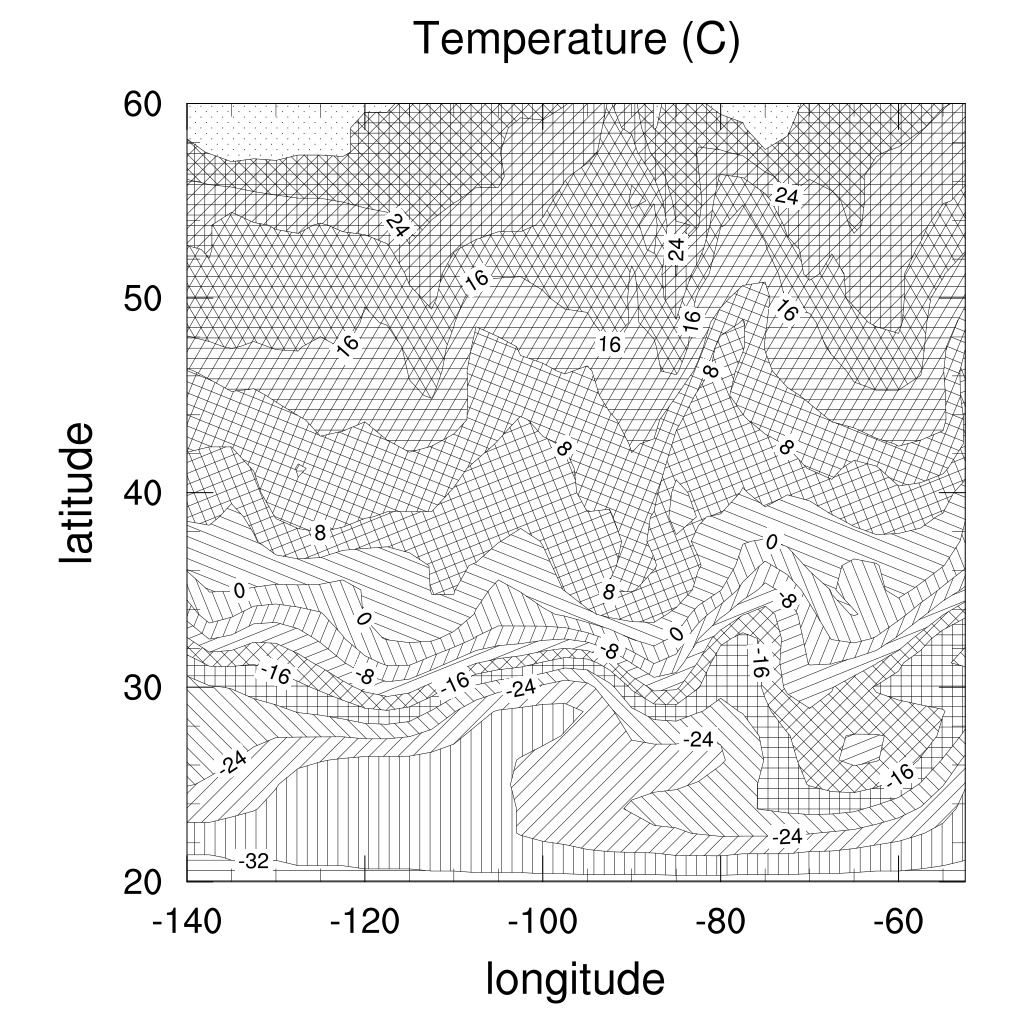
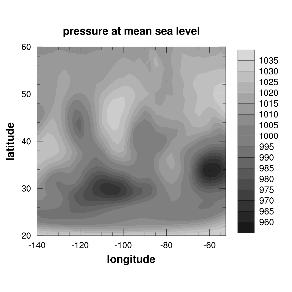
#---------- Begin fifth plot ------------------------------------------
Draw a contour plot of the pres variable and fill the contour lines in solid colors using a grayscale color map that you define yourself.
  cmap = numpy.array([[0.00, 0.00, 0.00], [1.00, 1.00, 1.00], \
                      [0.10, 0.10, 0.10], [0.15, 0.15, 0.15], \
                      [0.20, 0.20, 0.20], [0.25, 0.25, 0.25], \
                      [0.30, 0.30, 0.30], [0.35, 0.35, 0.35], \
                      [0.40, 0.40, 0.40], [0.45, 0.45, 0.45], \
                      [0.50, 0.50, 0.50], [0.55, 0.55, 0.55], \
                      [0.60, 0.60, 0.60], [0.65, 0.65, 0.65], \
                      [0.70, 0.70, 0.70], [0.75, 0.75, 0.75], \
                      [0.80, 0.80, 0.80], [0.85, 0.85, 0.85]],'f')
For this plot, use grayscale values to fill the contour levels. To do this, you need to define your own color map. Color maps are represented by NumPy arrays of red, green, and blue float values (referred to as RGB values) ranging from 0. to 1. (to indicate the intensity of that particular color). The first entry in a color map is the background color, and the second entry is the foreground color. To get a color map of grayscale values, use equal values for R, G, and B.
For more information on creating your own color map, see the section on "Color maps".
  rlist.wkColorMap = cmap
  Ngl.set_values(wks,rlist)
Again, we're using the PyNGL function Ngl.set_values to change the value of the color map, this time to a color map we've defined ourselves.
  if hasattr(pres,"long_name"):
    resources.tiMainString = pres.long_name
Change the title to reflect the new data you are contouring.
presa = pres[0,:,:]
Read the data for the pressure field pres into a NumPy array.
  if hasattr(pres,"_FillValue"):
    presa = (0.01*presa*numpy.not_equal(presa,pres._FillValue)) +   \
          pres._FillValue*numpy.equal(presa,pres._FillValue)
  else:
    presa = 0.01*presa
These calculations convert the presa array from to millibars. If pres has a _FillValue set, then we have to make sure that those values are not converted; if pres does not have a _FillValue set, then the conversion can be done without care for missing values.
plot = Ngl.contour(wks,presa,resources) # Draw a contour plot.
Draw the contour plot of the pressure variable.
  print "\nSubset [2:6,7:10] of temp array:" # Print subset of "temp" variable.
  print tempa[2:6,7:10]
  print "\nDimensions of temp array:"        # Print dimension names of T.
  print temp.dimensions
  print "\nThe long_name attribute of T:"    # Print the long_name attribute of T.
  print temp.long_name
  print "\nThe nlat data:"                   # Print the lat data.
  print lat[:]
  print "\nThe nlon data:"                   # Print the lon data.
  print lon[:]
Print some various properties of the netCDF variables.
  os.system("/bin/rm -f data.asc")
  sys.stdout = open("data.asc","w")
  for i in range(7,2,-2):
    for j in range(0,5):
      print "%9.5f" % (tempa[i,j])
Write a subsection of tempa to an ASCII file.
Ngl.end()
Required to end the script.