PyNGL/PyNIO tutorial: example 6 - vector plots over maps

PyNGL > tutorial examples > 1 | 2 | 3 | 4 | 5 | 6 | 7 | 8 | 9 | 10 | 11

Example 6 - vector plots over maps

This example reads in some netCDF files and creates three vector plots over different map projections. Resources are used to change aspects of both the vectors and the maps. To find out more about netCDF, see http://my.unidata.ucar.edu/content/software/netcdf/

To run this example, you must have Numerical Python installed in your Python implementation. Numerical Python (also known as "NumPy") is a Python module allowing for efficient array processing.

This example reads in a netCDF file, so you will need to have the Nio module (this module comes with PyNGL). netCDF is a self-documenting and network-transparent data format - see the netCDF User Guide for details.

There are two ways to run this example:

execute

    pynglex ngl06p

or download

ngl06p.py

and type:

python ngl06p.py

Output from example 6

Frame 1	Frame 2	Frame 3

(Click on any frame to see it enlarged.)

  0. #
  1. #  Import NumPy.
  2. #
  3. import numpy
  4. 
  5. #
  6. #  Import the NetCDF reader.
  7. #
  8. import Nio
  9. 
 10. #
 11. #  Import PyNGL support functions.
 12. #
 13. import Ngl
 14. #
 15. #  Open netCDF files.
 16. #
 17. dirc = Ngl.pynglpath("data")
 18. 
 19. #
 20. #  Open the netCDF file.
 21. #
 22. ufile = Nio.open_file(dirc + "/cdf/Ustorm.cdf","r")
 23. vfile = Nio.open_file(dirc + "/cdf/Vstorm.cdf","r")
 24. tfile = Nio.open_file(dirc + "/cdf/Tstorm.cdf","r")
 25. 
 26. #
 27. #  Get the u/v variables.
 28. #
 29. u = ufile.variables["u"]
 30. v = vfile.variables["v"]
 31. lat = ufile.variables["lat"]
 32. lon = ufile.variables["lon"]
 33. ua = u[0,:,:]
 34. va = v[0,:,:]
 35. 
 36. wks_type = "ps"
 37. wks = Ngl.open_wks(wks_type,"ngl06p")
 38. 
 39. #----------- Begin first plot -----------------------------------------
 40. 
 41. resources = Ngl.Resources()
 42. if hasattr(u,"_FillValue"):
 43.   resources.vfMissingUValueV = u._FillValue
 44. if hasattr(v,"_FillValue"):
 45.   resources.vfMissingVValueV = v._FillValue
 46. 
 47. nlon = len(lon)
 48. nlat = len(lat)
 49. resources.vfXCStartV  = float(lon[0])             # Define X/Y axes range
 50. resources.vfXCEndV    = float(lon[len(lon[:])-1]) # for vector plot.
 51. resources.vfYCStartV  = float(lat[0])
 52. resources.vfYCEndV    = float(lat[len(lat[:])-1])
 53. 
 54. map = Ngl.vector_map(wks,ua,va,resources)  # Draw a vector plot of u and v
 55. 
 56. #----------- Begin second plot -----------------------------------------
 57. 
 58. cmap = numpy.array([[1.00, 1.00, 1.00], [0.00, 0.00, 0.00], \
 59.                     [.560, .500, .700], [.300, .300, .700], \
 60.                     [.100, .100, .700], [.000, .100, .700], \
 61.                     [.000, .300, .700], [.000, .500, .500], \
 62.                     [.000, .700, .100], [.060, .680, .000], \
 63.                     [.550, .550, .000], [.570, .420, .000], \
 64.                     [.700, .285, .000], [.700, .180, .000], \
 65.                     [.870, .050, .000], [1.00, .000, .000], \
 66.                     [.700, .700, .700]],'f')
 67. 
 68. rlist = Ngl.Resources()
 69. rlist.wkColorMap = cmap
 70. Ngl.set_values(wks,rlist)
 71. 
 72. resources.mpLimitMode       = "Corners"  # Zoom in on the plot area.
 73. resources.mpLeftCornerLonF  = float(lon[0])
 74. resources.mpRightCornerLonF = float(lon[len(lon[:])-1])
 75. resources.mpLeftCornerLatF  = float(lat[0])
 76. resources.mpRightCornerLatF = float(lat[len(lat[:])-1])
 77. 
 78. resources.mpPerimOn         =   True    # Turn on map perimeter.
 79. 
 80. resources.vpXF      = 0.1   # Increase size and change location
 81. resources.vpYF      = 0.92  # of vector plot.
 82. resources.vpWidthF  = 0.75
 83. resources.vpHeightF = 0.75
 84. 
 85. resources.vcMonoLineArrowColor = False  # Draw vectors in color.
 86. resources.vcMinFracLengthF     = 0.33   # Increase length of
 87. resources.vcMinMagnitudeF      = 0.001  # vectors.
 88. resources.vcRefLengthF         = 0.045
 89. resources.vcRefMagnitudeF      = 20.0
 90. 
 91. map = Ngl.vector_map(wks,ua,va,resources)  # Draw a vector plot.
 92. 
 93. #----------- Begin third plot -----------------------------------------
 94. tfile = Nio.open_file(dirc+"/cdf/Tstorm.cdf","r")    # Open a netCDF file.
 95. temp = tfile.variables["t"]
 96. tempa = temp[0,:,:]
 97. if hasattr(temp,"_FillValue"):
 98.   tempa = ((tempa-273.15)*9.0/5.0+32.0) *  \
 99.           numpy.not_equal(tempa,temp._FillValue) + \
100.           temp._FillValue*numpy.equal(tempa,temp._FillValue)
101.   resources.sfMissingValueV = temp._FillValue
102. else:
103.   tempa = (tempa-273.15)*9.0/5.0+32.0
104. 
105. temp_units = "(deg F)"
106. 
107. resources.mpProjection = "Mercator"  # Change the map projection.
108. resources.mpCenterLonF = -100.0
109. resources.mpCenterLatF =   40.0
110. 
111. resources.mpLimitMode  = "LatLon"  # Change the area of the map
112. resources.mpMinLatF    =  18.0     # viewed.
113. resources.mpMaxLatF    =  65.0
114. resources.mpMinLonF    = -128.
115. resources.mpMaxLonF    = -58.
116. 
117. resources.mpFillOn               = True  # Turn on map fill.
118. resources.mpLandFillColor        = 16    # Change land color to grey.
119. resources.mpOceanFillColor       = -1    # Change oceans and inland
120. resources.mpInlandWaterFillColor = -1    # waters to transparent.
121. 
122. resources.mpGridMaskMode         = "MaskNotOcean"  # Draw grid over ocean.
123. resources.mpGridLineDashPattern  = 2
124. resources.vcFillArrowsOn           = True  # Fill the vector arrows
125. resources.vcMonoFillArrowFillColor = False # using multiple colors.
126. resources.vcFillArrowEdgeColor     = 1     # Draw the edges in black.
127. 
128. resources.tiMainString      = "~F25~Wind velocity vectors"  # Title
129. resources.tiMainFontHeightF = 0.03
130. 
131. resources.pmLabelBarDisplayMode  = "Always"       # Turn on a label bar.
132. resources.pmLabelBarSide         = "Bottom"       # Change orientation
133. resources.lbOrientation          = "Horizontal"   # Orientation of label bar.
134. resources.lbTitleString          = "TEMPERATURE (~S~o~N~F)"
135. 
136. resources.mpOutlineBoundarySets = "GeophysicalAndUSStates"
137. 
138. map = Ngl.vector_scalar_map(wks,ua[::2,::2],va[::2,::2],  \
139.                             tempa[::2,::2],resources)
140. 
141. del map
142. del u
143. del v
144. del temp
145. del tempa
146. 
147. Ngl.end()

Explanation of example 6

Line 3:

  import numpy

Import the Numerical Python module. You must have this module installed in your Python implementation. This module is used for efficient array processing. The names of the functions in the Numerical Python package are not exposed by this import, meaning that all functions and attributes in that package will have to be qualified with "numpy".

The Numerical Python package is also known as "NumPy".

Line 8:

  import Nio

Import the Nio module for a netCDF reader. This module comes with the PyNGL package. netCDF is a self-documenting and network-transparent data format - see the netCDF User Guide for details.

Line 13:

  import Ngl

Import all of the Ngl functions. The Ngl module must be on your Python search path.

Line 17:

  dirc = Ngl.pynglpath("data")

The built-in function Ngl.pynglpath returns the full pathname for a given PyNGL system directory, or the default value for a particular internal parameter.

Lines 22-24:

  ufile = Nio.open_file(dirc + "/cdf/Ustorm.cdf","r")
  vfile = Nio.open_file(dirc + "/cdf/Vstorm.cdf","r")
  tfile = Nio.open_file(dirc + "/cdf/Tstorm.cdf","r")

These lines open three different netCDF files in read only mode.

Lines 29-32:

  u = ufile.variables["u"]
  v = vfile.variables["v"]
  lat = ufile.variables["lat"]
  lon = ufile.variables["lon"]

These assignments associate Python NumPy objects with netCDF variables. No data is actually read in making these assignments.

Lines 33-34:

  ua = u[0,:,:]
  va = v[0,:,:]

u and v are references to 3-dimensional arrays (of the same size) of wind velocity vector data, where the first dimension represents time, the second dimension represents latitude, and the third dimension represents longitude. The above lines read the first time step of u/v data into NumPy arrays.

Line 39:

  #----------- Begin first plot -----------------------------------------

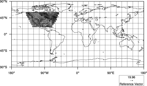
Draw a vector plot over a map, using the default map projection (cylindrical equidistant). The only resources set for this plot are for determining where on the map the vector plot should be overlaid.

Lines 41-45:

  resources = Ngl.Resources()
  if hasattr(u,"_FillValue"):
    resources.vfMissingUValueV = u._FillValue
  if hasattr(v,"_FillValue"):
    resources.vfMissingVValueV = v._FillValue

Specify the vector field missing values for u and v if such values are attributes of the netCDF variables.

Lines 47-52:

  nlon = len(lon)
  nlat = len(lat)
  resources.vfXCStartV  = lon[0][0]             # Define X/Y axes range
  resources.vfXCEndV    = lon[len(lon[:])-1][0] # for vector plot.
  resources.vfYCStartV  = lat[0][0]
  resources.vfYCEndV    = lat[len(lat[:])-1][0]

Set some VectorField resources to define the two corners of the latitude/longitude rectangle to overlay the vector plot on. A more detailed description of overlaying plots on a map plot is in example 5, which explains the overlay process of a contour plot on a map using ScalarField resources. The same explanation applies to the VectorField resources used here. The VectorField resources themselves are described in more detail in example 3.

Line 54:

  map = Ngl.vector_map(wks,ua,va,resources)  # Draw a vector plot of u and v

Create and draw a vector plot of the ua and va arrays over a map. The default map projection is cylindrical equidistant. The first argument of the Ngl.vector_map function is the workstation variable returned from the previous call to Ngl.open_wks(. The next two arguments represent the 2-dimensional vector field to be plotted (they must have the same dimensions and can be of NumPy type float, double, or integer). The last argument is the resource list.

Note that the vector plot covers only a small area of the map. This is because the latitude values you specified above only go from 20 to 60 in latitude and from -140 to -52.5 in longitude. These latitude/longitude values roughly cover the area which is the United States, so this is where you'll see the vector plot overlaid.

As described in example 5 for Ngl.contour_map, the Ngl.vector_map function creates two plots, the vector plot and the map plot. The map plot object is what's returned from the function.

Line 56:

  #----------- Begin second plot -----------------------------------------

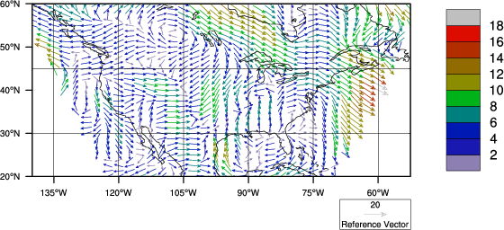
Zoom in on the area of the map that contains the vector plot, draw the vectors in color and make them larger, and increase the size of the plot within the viewport

Lines 58-66:

  cmap = numpy.array([[1.00, 1.00, 1.00], [0.00, 0.00, 0.00], \
                      [.560, .500, .700], [.300, .300, .700], \
                      [.100, .100, .700], [.000, .100, .700], \
                      [.000, .300, .700], [.000, .500, .500], \
                      [.000, .700, .100], [.060, .680, .000], \
                      [.550, .550, .000], [.570, .420, .000], \
                      [.700, .285, .000], [.700, .180, .000], \
                      [.870, .050, .000], [1.00, .000, .000], \
                      [.700, .700, .700]],'f')

Lines 68-70:

  rlist = Ngl.Resources()
  rlist.wkColorMap = cmap
  Ngl.set_values(wks,rlist)

Associate the new color map with the output workstation.

Lines 72-76:

  resources.mpLimitMode       = "Corners"  # Zoom in on the plot area.
  resources.mpLeftCornerLonF  = lon[0][0]
  resources.mpRightCornerLonF = lon[len(lon[:])-1][0]
  resources.mpLeftCornerLatF  = lat[0][0]
  resources.mpRightCornerLatF = lat[len(lat[:])-1][0]

Set some resources to zoom in on the area of the map where the vectors are concentrated. Use the same bounds that you used to define the area that the vector plot is overlaid on.

Lines 80-83:

  resources.vpXF      = 0.1   # Increase size and change location
  resources.vpYF      = 0.92  # of vector plot.
  resources.vpWidthF  = 0.75
  resources.vpHeightF = 0.75

Set some resources to change the size and position of the plot you want to draw in the viewport. The viewport is discussed in more detail in example 5.

Create and draw a vector plot of ua and va over a map. This time you should be able to see the vector plot better since you zoomed in on the area of the map containing the vectors.

Lines 85-89:

  resources.vcMonoLineArrowColor = False  # Draw vectors in color.
  resources.vcMinFracLengthF     = 0.33   # Increase length of
  resources.vcMinMagnitudeF      = 0.001  # vectors.
  resources.vcRefLengthF         = 0.045
  resources.vcRefMagnitudeF      = 20.0

Set some resources to draw the vectors in color and to increase their lengths. The above resources are described in more detail in example 3. The default color map is used in this case.

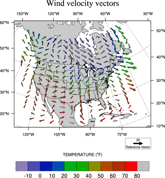
Create your own color map, draw filled vectors instead of line vectors, color the vectors according to a temperature scalar field, change the map projection, fill land in gray, mask the map grid over land, thin the vectors, and draw a label bar at the bottom of the plot.

Line 91:

  map = Ngl.vector_map(wks,ua,va,resources)  # Draw a vector plot.

Set some resources to change the size and position of the plot you want to draw in the viewport. The viewport is discussed in more detail in example 5.

Create and draw a vector plot of ua and va over a map. This time you should be able to see the vector plot better since you zoomed in on the area of the map containing the vectors.

Line 93:

  #----------- Begin third plot -----------------------------------------

Set some resources to draw the vectors in color and to increase their lengths. The above resources are described in more detail in example 3. The default color map is used in this case.

Line 94:

  tfile = Nio.open_file(dirc+"/cdf/Tstorm.cdf","r")    # Open a netCDF file.

Open another netCDF file.

Line 95-96:

  temp = tfile.variables["t"]
  tempa = temp[0,:,:]

Read the first time step of the temperature data into the NumPy array tempa.

Lines 97-103:

  if hasattr(temp,"_FillValue"):
    tempa = ((tempa-273.15)*9.0/5.0+32.0) *  \
            numpy.not_equal(tempa,temp._FillValue) + \
            temp._FillValue*numpy.equal(tempa,temp._FillValue)
    resources.sfMissingValueV = temp._FillValue
  else:
    tempa = (tempa-273.15)*9.0/5.0+32.0

Convert the temperatures from Kelvin to Fahrenheit, making sure that the missing value remains unchanged.

Lines 107-109:

  resources.mpProjection = "Mercator"  # Change the map projection.
  resources.mpCenterLonF = -100.0
  resources.mpCenterLatF =   40.0

Change the map projection to "Mercator" and change the center longitude and latitude values to be the approximate center of the latitude/longitude rectangle you're about to define when you set the mpLimitMode resource.

Lines 111-115:

  resources.mpLimitMode  = "LatLon"  # Change the area of the map
  resources.mpMinLatF    =  18.0     # viewed.
  resources.mpMaxLatF    =  65.0
  resources.mpMinLonF    = -128.
  resources.mpMaxLonF    = -58.

Change the mode for zooming in on the map projection to "LatLon". When mpLimitMode is set to this string, the resources mpMinLatF, mpMaxLatF, mpMinLonF, and mpMaxLonF are used to determine the limits of the maximum viewable portion of the map in latitude/longitude coordinates.

Lines 117-120:

  resources.mpFillOn               = True  # Turn on map fill.
  resources.mpLandFillColor        = 16    # Change land color to grey.
  resources.mpOceanFillColor       = -1    # Change oceans and inland
  resources.mpInlandWaterFillColor = -1    # waters to transparent.

Turn on the filling of map geographical areas, and fill the land gray and the oceans and inland water transparent. Note that this method is different that the one used in example 5 where the map areas you wanted to fill were specified with the resource mpFillColors. Either method could have been used in this case, since you filling the same types of areas.

Lines 122-123:

  resources.mpGridMaskMode         = "MaskNotOcean"  # Draw grid over ocean.
  resources.mpGridLineDashPattern  = 2

Draw the map latitude/longitude grid lines over the ocean only, and use a dashed line to draw the grid (the default is a solid line).

Lines 124-126:

  resources.vcFillArrowsOn           = True  # Fill the vector arrows
  resources.vcMonoFillArrowFillColor = False # using multiple colors.
  resources.vcFillArrowEdgeColor     = 1     # Draw the edges in black.

Set some resources to indicate that you want multi-colored filled vector arrows and the edges of the arrows drawn in the foreground color. By default, the edges of the arrows are drawn in the background color.

Lines 131-134:

  resources.pmLabelBarDisplayMode  = "Always"       # Turn on a label bar.
  resources.pmLabelBarSide         = "Bottom"       # Change orientation
  resources.lbOrientation          = "Horizontal"   # Orientation of label bar.
  resources.lbTitleString          = "TEMPERATURE (~S~o~N~F)"

Turn on the drawing of a label bar, title it, and put it at the bottom of the plot. The text function code "~S~o~N~F" draws an "o" as a superscript character before the letter "F", to indicate "degrees Fahrenheit."

Line 136:

  resources.mpOutlineBoundarySets = "GeophysicalAndUSStates"

The mpOutlineBoundarySets resource allows you to indicate what kind of map outlines to draw. Using a value of "GeophysicalAndUSStates" draws outlines of all global geophysical features and also U.S. States and inland water features. The default of mpOutlineBoundarySets is "Geophysical."

Lines 138-139:

  map = Ngl.vector_scalar_map(wks,ua[::2,::2],va[::2,::2],  \
                              tempa[::2,::2],resources)

Use the Ngl.vector_scalar_map function to draw a vector plot over a map and color the vectors according to the scalar field tempa. The Ngl.vector_scalar_map function is the same as the Ngl.vector_map function, only it has a scalar field as an additional argument (the fourth argument). The scalar field must be the same dimensions as the U and V arrays.

In the call to Ngl.vector_scalar_map, the syntax "::2" is being used to "thin" the vectors; that is, only every other data point is passed on to the plotting function.