
PyNGL > tutorial examples > 1 | 2 | 3 | 4 | 5 | 6 | 7 | 8 | 9 | 10 | 11
Example 3 - vector plots
This example reads in three netCDF files and creates four vector plots, using data from all three files. Resources are used to change aspects of each vector plot.To find out more about netCDF, see http://my.unidata.ucar.edu/content/software/netcdf/.
To run this example, you must have Numerical Python installed in your Python implementation. Numerical Python (also known as "NumPy") is a Python module allowing for efficient array processing. This example reads in a netCDF file, so you will need to have the Nio module (this module comes with PyNGL). netCDF is a self-documenting and network-transparent data format - see the netCDF User Guide for details.
There are two ways to run this example:
execute
pynglex ngl03p
or
download
ngl03p.pyand type:
python ngl03p.py
Output from example 3
| Frame 1 | Frame 2 | Frame 3 | Frame 4 |
|---|---|---|---|
| 
| 
| 
|
(Click on any frame to see it enlarged.)
  0. #
  1. #  Import NumPy.
  2. #
  3. import numpy
  4.
  5. #
  6. #  Import Nio.
  7. #
  8. import Nio
  9.
 10. #
 11. #  Import Ngl support functions.
 12. #
 13. import Ngl
 14. #
 15. #  Open the netCDF files.
 16. #
 17. dirc  = Ngl.pynglpath("data")
 18. ufile = Nio.open_file(dirc + "/cdf/Ustorm.cdf","r")  # Open two netCDF files.
 19. vfile = Nio.open_file(dirc + "/cdf/Vstorm.cdf","r")
 20.
 21. #
 22. #  Get the u/v variables.
 23. #
 24. u = ufile.variables["u"]
 25. v = vfile.variables["v"]
 26. lat = ufile.variables["lat"]
 27. lon = ufile.variables["lon"]
 28. ua = u[0,:,:]
 29. va = v[0,:,:]
 30.
 31. wks_type = "ps"
 32. wks = Ngl.open_wks(wks_type,"ngl03p")
 33.
 34. resources = Ngl.Resources()
 35. if hasattr(u,"_FillValue"):
 36.   resources.vfMissingUValueV = u._FillValue
 37. if hasattr(v,"_FillValue"):
 38.   resources.vfMissingVValueV = v._FillValue
 39.
 40. vc = Ngl.vector(wks,ua,va,resources)
 41.
 42. #----------- Begin second plot -----------------------------------------
 43.
 44. resources.vcMinFracLengthF = 0.33
 45. resources.vcRefMagnitudeF  = 20.0
 46. resources.vcRefLengthF     = 0.045
 47. resources.vcMonoLineArrowColor  = False   # Draw vectors in color.
 48.
 49. vc = Ngl.vector(wks,ua,va,resources)
 50.
 51. #----------- Begin third plot -----------------------------------------
 52.
 53. resources.tiMainString  = "~F22~wind velocity vectors - January 1996"
 54. resources.tiXAxisString = "longitude"
 55. resources.tiYAxisString = "latitude"
 56.
 57. resources.vfXCStartV  = float(lon[0])            # Define X/Y axes range
 58. resources.vfXCEndV    = float(lon[len(lon[:])-1]) # for vector plot.
 59. resources.vfYCStartV  = float(lat[0])
 60. resources.vfYCEndV    = float(lat[len(lat[:])-1])
 61.
 62. vc = Ngl.vector(wks,ua,va,resources)
 63.
 64. #---------- Begin fourth plot ------------------------------------------
 65.
 66. tfile = Nio.open_file(dirc+"/cdf/Tstorm.cdf","r")    # Open a netCDF file.
 67. temp = tfile.variables["t"]
 68.
 69. tempa = temp[0,:,:]
 70. #
 71. #  Convert from degrees Kelvin to degrees F.
 72. #  If the data has a fill value, do the conversion  at those
 73. #  values not equal to the fill value and fill in with the fill
 74. #  value elsewhere.
 75. #
 76. if hasattr(temp,"_FillValue"):
 77.   tempa = ((tempa-273.15)*9.0/5.0+32.0) *  \
 78.           numpy.not_equal(tempa,temp._FillValue) + \
 79.           temp._FillValue*numpy.equal(tempa,temp._FillValue)
 80.   resources.sfMissingValueV = temp._FillValue
 81. else:
 82.   tempa = (tempa-273.15)*9.0/5.0+32.0
 83.
 84. temp_units = "(deg F)"
 85.
 86. cmap = numpy.array([[1.00, 1.00, 1.00], [0.00, 0.00, 0.00], \
 87.                     [.560, .500, .700], [.300, .300, .700], \
 88.                     [.100, .100, .700], [.000, .100, .700], \
 89.                     [.000, .300, .700], [.000, .500, .500], \
 90.                     [.000, .700, .100], [.060, .680, .000], \
 91.                     [.550, .550, .000], [.570, .420, .000], \
 92.                     [.700, .285, .000], [.700, .180, .000], \
 93.                     [.870, .050, .000], [1.00, .000, .000], \
 94.                     [.700, .700, .700]],'f')
 95.
 96. rlist = Ngl.Resources()
 97. rlist.wkColorMap = cmap
 98. Ngl.set_values(wks,rlist)
 99.
100. resources.vcFillArrowsOn           = True  # Fill the vector arrows
101. resources.vcMonoFillArrowFillColor = False # in different colors
102. resources.vcFillArrowEdgeColor     = 1     # Draw the edges in black.
103. resources.vcFillArrowWidthF        = 0.055 # Make vectors thinner.
104.
105. resources.tiMainString      = "~F22~wind velocity vectors colored by temperature " + temp_units
106. resources.tiMainFontHeightF = 0.02  # Make font slightly smaller.
107.
108. vc = Ngl.vector_scalar(wks,ua,va,tempa,resources) # Draw a vector plot of
109.
110. del vc
111. del u
112. del v
113. del temp
114. del tempa
115.
116. Ngl.end()
Explanation of example 3
Line 3:
import numpy
Import the Numerical Python module. You must have this module installed in your Python implementation. This module is used for efficient array processing. The names of the functions in the Numerical Python package are not exposed by this import, meaning that all functions and attributes in that package will have to be qualified with "numpy".
The Numerical Python package is also known as "NumPy".
import Nio
Import the Nio module for a netCDF reader. This module comes with the PyNGL package). netCDF is a self-documenting and network-transparent data format - see the netCDF User Guide for details.
import Ngl
Import all of the Ngl functions. The Ngl module must be on your Python search path.
dirc = Ngl.pynglpath("data")
The built-in function Ngl.pynglpath returns the full pathname for a given PyNGL system directory, or the default value for a particular internal parameter.
  ufile = Nio.open_file(dirc + "/cdf/Ustorm.cdf","r")  # Open two netCDF files.
  vfile = Nio.open_file(dirc + "/cdf/Vstorm.cdf","r")
This lines open sample netCDF files for reading.
  u = ufile.variables["u"]
  v = vfile.variables["v"]
  lat = ufile.variables["lat"]
  lon = ufile.variables["lon"]
These assignments associate Python NumPy objects with netCDF variables. No data is actually read in making these assignments.
  ua = u[0,:,:]
  va = v[0,:,:]
These lines read data from the netCDF variables into NumPy arrays.
  wks_type = "ps"
  wks = Ngl.open_wks(wks_type,"ngl03p")
Open a workstation for drawing the vector plots.
resources = Ngl.Resources()
Get ready to set up a list of resources for changing the look of the plot. See example 1 for an explanation of how resources are set. Vector plot resources are part of the "VectorPlot" group and all start with the letters "vc". They are documented in the VectorPlot resource descriptions section.
Data associated with a vector plot is called a "VectorField." VectorField resources start with "vf" and are documented in the VectorField resource descriptions section.
  if hasattr(u,"_FillValue"):
    resources.vfMissingUValueV = u._FillValue
  if hasattr(v,"_FillValue"):
    resources.vfMissingVValueV = v._FillValue
These lines set the U and V missing values for the vector field data based on the values in the netCDF files.
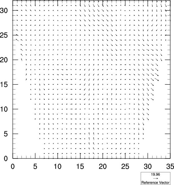
vc = Ngl.vector(wks,ua,va,resources)
Create and draw a vector plot of the 2-dimensional arrays u and v. The first argument of the Ngl.vector function is the workstation object returned from the previous call to Ngl.open_wks. The next two arguments represent the 2-dimensional vector field to be vectorized (they must have the same dimensions, be of a NumPy type float, double, or integer, and be ordered Y x X). The last argument is the resource list indicating values that you have set that modify the plot.
The default vector plot drawn contains labeled tick marks and a "reference vector" label at the bottom right of the plot. Since no ranges have been defined for the X and Y axes in this plot, the range values default to 0 to n-1, where n is the number of points in that dimension. By default, vectors are drawn with lines and hollow arrow heads, but you can change them to filled vectors as you'll see in a later frame in this example.
Note that there are some areas in the vector plot where no vectors are drawn. This is due to the presence of the missing values in the data.
#----------- Begin second plot -----------------------------------------
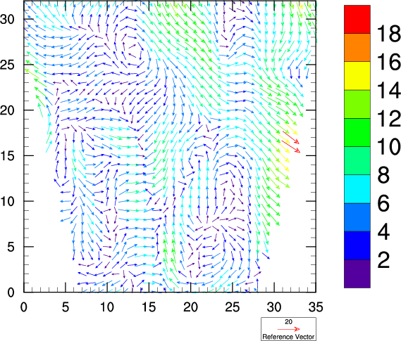
Draw the same vector plot, only this time set some resources to change the length of the vectors and draw them in color.
resources.vcMinFracLengthF = 0.33
The vcMinFracLengthF resource sets the length of the minimum magnitude vector as a fraction of the length of the reference vector (the default is 0).
  resources.vcRefMagnitudeF  = 20.0
  resources.vcRefLengthF     = 0.045
  resources.vcMonoLineArrowColor  = False   # Draw vectors in color.
The vcRefMagnitudeF resource indicates which magnitude to use for the reference magnitude (the default is 0, a special value that indicates that the maximum magnitude in the vector field is used as a reference magnitude). vcRefLengthF sets the length of the reference magnitude in NDC coordinates (this resource is normally set dynamically according to the number of elements in the vector field and the size of the plot's viewport).
vc = Ngl.vector(wks,ua,va,resources)
Draw the new vector plot using the resources you just set.
#----------- Begin third plot -----------------------------------------
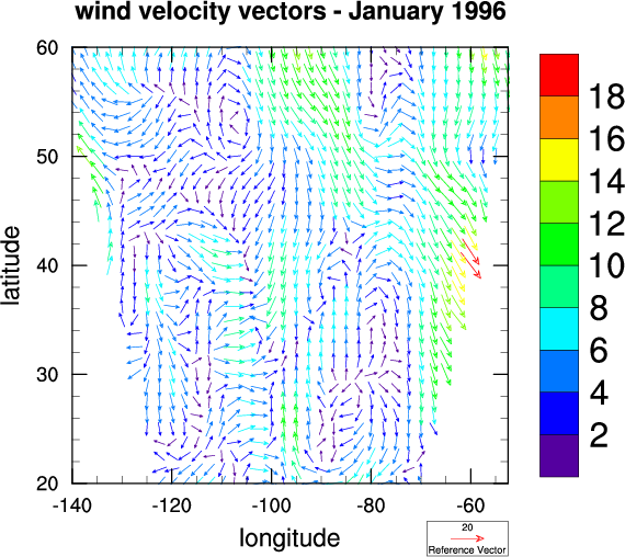
Draw the same vector plot, only set some resources to change the the X and Y axis ranges, and add a label bar and a title.
  resources.tiMainString  = "~F22~wind velocity vectors - January 1996"
  resources.tiXAxisString = "longitude"
  resources.tiYAxisString = "latitude"
Create a title and labels for the X and Y axes. PyNGNGL allows special text functions to be embedded in strings to indicate you want things like sub/superscripting, different fonts, carriage returns, etc. By default, each special function is preceded and succeeded with a tilde (~). In the string for the tiMainString resource, the "~F22~" part is a text function indicating that you want to use font 22, which is Helvetica-bold.
If you happen to have a tilde as part of the string, and you don't want it to be interpreted as a function code, then you can use the txFuncCode resource to change the function code character. The various text function codes are documented in the "Text function codes" section.
  resources.vfXCStartV  = lon[0][0]            # Define X/Y axes range
  resources.vfXCEndV    = lon[len(lon[:])-1][0] # for vector plot.
  resources.vfYCStartV  = lat[0][0]
  resources.vfYCEndV    = lat[len(lat[:])-1][0]
The resources vfXCStartV and vfXCEndV indicate the starting and ending data locations along the X axis of the vector field you are plotting. Likewise, vfYCStartV and vfYCEndV indicate the starting and ending data locations along the Y axis of the vector field. If you don't set these resources, then the vf*StartV resources default to 0.0 and the vf*EndV resources default to the number of data elements in that direction minus 1.
vc = Ngl.vector(wks,ua,va,resources)
Draw the third vector plot with the new resources that you added.
#---------- Begin fourth plot ------------------------------------------
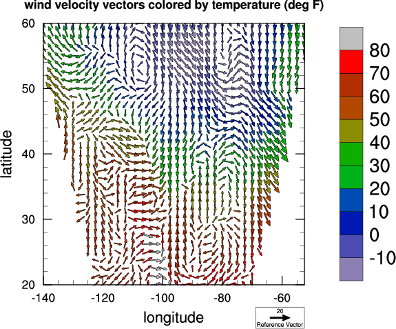
Create your own color map, color the vectors according to a separate temperature scalar field, and fill the vector arrows.
  tfile = Nio.open_file(dirc+"/cdf/Tstorm.cdf","r")    # Open a netCDF file.
  temp = tfile.variables["t"]

  tempa = temp[0,:,:]
Open a netCDF file containing temperature data, read in the first level of the temperature data
  if hasattr(temp,"_FillValue"):
    tempa = ((tempa-273.15)*9.0/5.0+32.0) *  \
            numpy.not_equal(tempa,temp._FillValue) + \
            temp._FillValue*numpy.equal(tempa,temp._FillValue)
    resources.sfMissingValueV = temp._FillValue
  else:
    tempa = (tempa-273.15)*9.0/5.0+32.0
Convert the temperatures from Kelvin to Fahrenheit making sure that the missing values retain their settings. The attribute _FillValue of the netCDF temperature variable is only an attribute of temp and not of tempa.
temp_units = "(deg F)"
Define the temperature units to be in degrees F for later use.
  cmap = numpy.array([[1.00, 1.00, 1.00], [0.00, 0.00, 0.00], \
                      [.560, .500, .700], [.300, .300, .700], \
                      [.100, .100, .700], [.000, .100, .700], \
                      [.000, .300, .700], [.000, .500, .500], \
                      [.000, .700, .100], [.060, .680, .000], \
                      [.550, .550, .000], [.570, .420, .000], \
                      [.700, .285, .000], [.700, .180, .000], \
                      [.870, .050, .000], [1.00, .000, .000], \
                      [.700, .700, .700]],'f')
Define your own color map. Details on creating your own color map are covered in example 2.
  rlist = Ngl.Resources()
  rlist.wkColorMap = cmap
  Ngl.set_values(wks,rlist)
These calls reset the color map of wks to cmap.
  resources.vcFillArrowsOn           = True  # Fill the vector arrows
  resources.vcMonoFillArrowFillColor = False # in different colors
  resources.vcFillArrowEdgeColor     = 1     # Draw the edges in black.
  resources.vcFillArrowWidthF        = 0.055 # Make vectors thinner.
Setting the vcFillArrowsOn resource to True produces filled vector arrows instead of vector arrows drawn with lines. Setting vcMonoFillArrowFillColor to False fills the vector arrows using multiple colors.
By default, the vcFillArrowEdgeColor resource is set to the background color (index 0). By changing this to the foreground color (index 1), you are making the vector arrows more visible. The vcFillArrowWidthF resource sets the width of the arrows as a fraction of the vcRefLengthF. The default is 0.1.
There's a handy vector arrow diagram in the description of VectorPlot that shows the various components of a vector arrow.
  resources.tiMainString      = "~F22~wind velocity vectors colored by temperature " + temp_units
  resources.tiMainFontHeightF = 0.02  # Make font slightly smaller.
Change the title for the plot and decrease the size of the font. Also, change the font of the title to 26 (Times-bold). Remember that predefined strings, like those listed in the font table, are case-insensitive and you could have specified the above fonts with "times-roman" or "HELVETICA" or any another combination of uppercase and lower case characters.
vc = Ngl.vector_scalar(wks,ua,va,tempa,resources) # Draw a vector plot of
Use the Ngl.vector_scalar function to draw a vector plot and color the vectors according to the scalar field temp. The Ngl.vector_scalar function is the same as the Ngl.vector function, only it has a scalar field as an additional argument (the fourth argument). The scalar field must have the same dimensions as the U and V arrays.
Ngl.end()
Required to end the script.